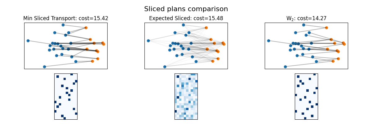
Sliced OT Plans

Compares different Sliced OT plans between two 2D point clouds. The min-Sliced transport plan was introduced in [85], and the Expected Sliced plan in [87], both were further studied theoretically in [86].

[85]

Mahey, G., Chapel, L., Gasso, G., Bonet, C., & Courty, N. (2023). Fast Optimal Transport through Sliced Generalized Wasserstein Geodesics. Advances in Neural Information Processing Systems, 36, 35350–35385.

[86]

Tanguy, E., Chapel, L., Delon, J. (2025). Sliced Transport Plans. arXiv preprint 2506.03661.

[87]

Liu, X., Diaz Martin, R., Bai Y., Shahbazi A., Thorpe M., Aldroubi A., Kolouri, S. (2024). Expected Sliced Transport Plans. International Conference on Learning Representations.

# Author: Eloi Tanguy <eloi.tanguy@math.cnrs.fr>
# License: MIT License

# sphinx_gallery_thumbnail_number = 1

Setup data and imports

import numpy as np

import ot
import matplotlib.pyplot as plt
from ot.sliced import get_random_projections


seed = 0
np.random.seed(seed)
n = 20
m = 10
d = 2
X = np.random.randn(n, 2)
Y = np.random.randn(m, 2) + np.array([5.0, 0.0])[None, :]
n_proj = 50
projections = get_random_projections(d, n_proj)
alpha = 0.3

Compute min-sliced transport plan

min_plan, min_cost, log_min = ot.min_sliced_transport_plan(
    X, Y, projections=projections, log=True
)

Compute Expected Sliced Plan

expected_plan, expected_cost, log_expected = ot.expected_sliced_plan(
    X, Y, projections=projections, log=True
)

Compute 2-Wasserstein Plan

a = np.ones(n, device=X.device) / n
b = np.ones(m, device=Y.device) / m
dists = ot.dist(X, Y)
W2 = ot.emd2(a, b, dists)
W2_plan = ot.emd(a, b, dists)

Plot resulting assignments

fig, axs = plt.subplots(2, 3, figsize=(12, 4))
fig.suptitle("Sliced plans comparison", y=0.95, fontsize=16)

# draw min sliced permutation
axs[0, 0].set_title(f"Min Sliced Transport: cost={min_cost:.2f}")
for i in range(X.shape[0]):
    for j in range(Y.shape[0]):
        if min_plan[i, j] > 0:
            axs[0, 0].plot(
                [X[i, 0], Y[j, 0]],
                [X[i, 1], Y[j, 1]],
                color="black",
                alpha=alpha,
            )
axs[1, 0].imshow(min_plan, interpolation="nearest", cmap="Blues")

# draw expected sliced plan
axs[0, 1].set_title(f"Expected Sliced: cost={expected_cost:.2f}")
for i in range(n):
    for j in range(m):
        w = alpha * expected_plan[i, j].item() * n
        axs[0, 1].plot(
            [X[i, 0], Y[j, 0]],
            [X[i, 1], Y[j, 1]],
            color="black",
            alpha=w,
            label="Expected Sliced plan" if i == 0 and j == 0 else None,
        )
axs[1, 1].imshow(expected_plan, interpolation="nearest", cmap="Blues")

# draw W2 plan
axs[0, 2].set_title(f"W$_2$: cost={W2:.2f}")
for i in range(n):
    for j in range(m):
        w = alpha * W2_plan[i, j].item() * n
        axs[0, 2].plot(
            [X[i, 0], Y[j, 0]],
            [X[i, 1], Y[j, 1]],
            color="black",
            alpha=w,
            label="W2 plan" if i == 0 and j == 0 else None,
        )
axs[1, 2].imshow(W2_plan, interpolation="nearest", cmap="Blues")

for ax in axs[0, :]:
    ax.scatter(X[:, 0], X[:, 1], label="X")
    ax.scatter(Y[:, 0], Y[:, 1], label="Y")

for ax in axs.flatten():
    ax.set_aspect("equal")
    ax.set_xticks([])
    ax.set_yticks([])

fig.tight_layout()

Compare Expected Sliced plans with different inverse-temperatures beta

As the temperature decreases, ES becomes sparser and approaches minPS

betas = [0.0, 5.0, 50.0]
n_plots = len(betas) + 1
size = 4
fig, axs = plt.subplots(2, n_plots, figsize=(size * n_plots, size))

fig.suptitle(
    "Expected Sliced plan varying $\\beta$ (inverse temperature)", y=0.95, fontsize=16
)
for beta_idx, beta in enumerate(betas):
    expected_plan, expected_cost = ot.expected_sliced_plan(
        X, Y, projections=projections, beta=beta
    )
    print(f"beta={beta}: cost={expected_cost:.2f}")

    axs[0, beta_idx].set_title(f"$\\beta$={beta}: cost={expected_cost:.2f}")
    for i in range(n):
        for j in range(m):
            w = alpha * expected_plan[i, j].item() * n
            axs[0, beta_idx].plot(
                [X[i, 0], Y[j, 0]],
                [X[i, 1], Y[j, 1]],
                color="black",
                alpha=w,
                label="Expected Sliced plan" if i == 0 and j == 0 else None,
            )

    axs[0, beta_idx].scatter(X[:, 0], X[:, 1], label="X")
    axs[0, beta_idx].scatter(Y[:, 0], Y[:, 1], label="Y")
    axs[1, beta_idx].imshow(expected_plan, interpolation="nearest", cmap="Blues")

# draw min sliced permutation (limit when beta -> +inf)
axs[0, -1].set_title(f"Min Sliced Transport: cost={min_cost:.2f}")
for i in range(X.shape[0]):
    for j in range(Y.shape[0]):
        if min_plan[i, j] > 0:
            axs[0, -1].plot(
                [X[i, 0], Y[j, 0]],
                [X[i, 1], Y[j, 1]],
                color="black",
                alpha=alpha,
            )

axs[0, -1].scatter(X[:, 0], X[:, 1], label="X")
axs[0, -1].scatter(Y[:, 0], Y[:, 1], label="Y")
axs[1, -1].imshow(min_plan, interpolation="nearest", cmap="Blues")

for ax in axs.flatten():
    ax.set_aspect("equal")
    ax.set_xticks([])
    ax.set_yticks([])

fig.tight_layout()

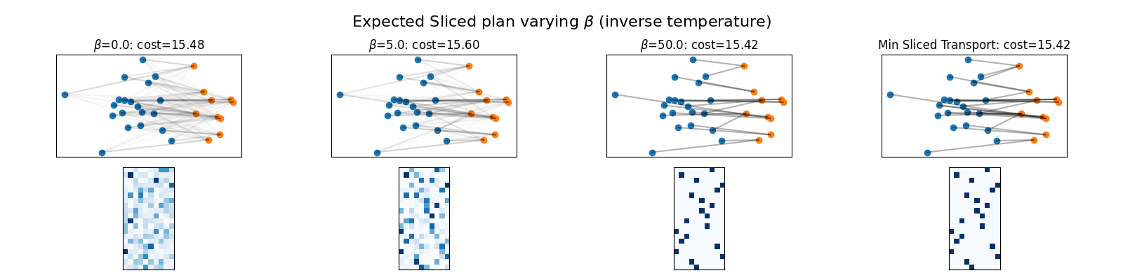
beta=0.0: cost=15.48
beta=5.0: cost=15.60
beta=50.0: cost=15.42