Sparse Optimal Transport

In many real-world optimal transport (OT) problems, the transport plan is naturally sparse: only a small fraction of all possible source-target pairs actually exchange mass. Using sparse OT solvers can provide significant computational speedups and memory savings compared to dense solvers.

This example demonstrates how to use sparse cost matrices with POT’s EMD solver, comparing sparse and dense formulations on both a minimal example and a larger concentric circles dataset.

# Author: Nathan Neike
#
# License: MIT License
# sphinx_gallery_thumbnail_number = 2

import numpy as np
import matplotlib.pyplot as plt
from scipy.sparse import coo_array
import ot

Example: concentric circles

n_clusters = 8
points_per_cluster = 25
n = n_clusters * points_per_cluster
k_neighbors = 8
rng = np.random.default_rng(0)

r_source = 1.0
r_target = 2.0
noise_scale = 0.06

theta = np.linspace(0.0, 2.0 * np.pi, n, endpoint=False)
cluster_labels = np.repeat(np.arange(n_clusters), points_per_cluster)

X_large = np.column_stack(
    [r_source * np.cos(theta), r_source * np.sin(theta)]
) + rng.normal(scale=noise_scale, size=(n, 2))
Y_large = np.column_stack(
    [r_target * np.cos(theta), r_target * np.sin(theta)]
) + rng.normal(scale=noise_scale, size=(n, 2))

a_large = np.zeros(n)
b_large = np.zeros(n)
for k in range(n_clusters):
    idx = np.where(cluster_labels == k)[0]
    a_large[idx] = 1.0 / n_clusters / points_per_cluster
    b_large[idx] = 1.0 / n_clusters / points_per_cluster

M_full = ot.dist(X_large, Y_large, metric="euclidean")

# Build sparse cost matrix: intra-cluster k-nearest neighbors
angles_X = np.arctan2(X_large[:, 1], X_large[:, 0])
angles_Y = np.arctan2(Y_large[:, 1], Y_large[:, 0])

rows = []
cols = []
vals = []
for k in range(n_clusters):
    src_idx = np.where(cluster_labels == k)[0]
    tgt_idx = np.where(cluster_labels == k)[0]
    for i in src_idx:
        diff = np.angle(np.exp(1j * (angles_Y[tgt_idx] - angles_X[i])))
        idx = np.argsort(np.abs(diff))[:k_neighbors]
        for j_local in idx:
            j = tgt_idx[j_local]
            rows.append(i)
            cols.append(j)
            vals.append(M_full[i, j])

M_sparse_large = coo_array((vals, (rows, cols)), shape=(n, n))
allowed_sparse = set(zip(rows, cols))

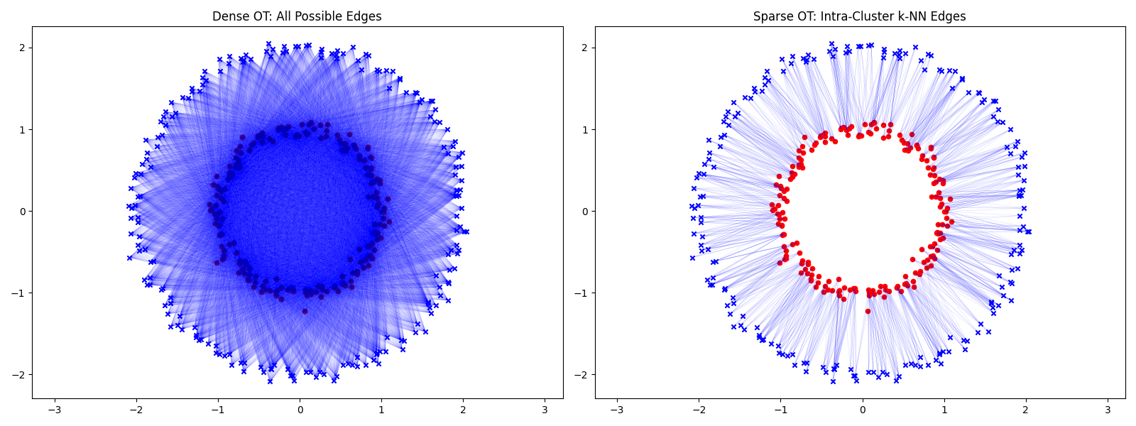
Visualize edge structures

plt.figure(figsize=(16, 6))

plt.subplot(1, 2, 1)
for i in range(n):
    for j in range(n):
        plt.plot(
            [X_large[i, 0], Y_large[j, 0]],
            [X_large[i, 1], Y_large[j, 1]],
            color="blue",
            alpha=0.2,
            linewidth=0.05,
        )
plt.scatter(X_large[:, 0], X_large[:, 1], c="r", marker="o", s=20)
plt.scatter(Y_large[:, 0], Y_large[:, 1], c="b", marker="x", s=20)
plt.axis("equal")
plt.title("Dense OT: All Possible Edges")

plt.subplot(1, 2, 2)
for i, j in allowed_sparse:
    plt.plot(
        [X_large[i, 0], Y_large[j, 0]],
        [X_large[i, 1], Y_large[j, 1]],
        color="blue",
        alpha=1,
        linewidth=0.05,
    )
plt.scatter(X_large[:, 0], X_large[:, 1], c="r", marker="o", s=20)
plt.scatter(Y_large[:, 0], Y_large[:, 1], c="b", marker="x", s=20)
plt.axis("equal")
plt.title("Sparse OT: Intra-Cluster k-NN Edges")

plt.tight_layout()
plt.show()

Solve and visualize transport plans

G_dense = ot.emd(a_large, b_large, M_full)
cost_dense = np.sum(G_dense * M_full)
print(f"Dense OT cost: {cost_dense:.6f}")

G_sparse, log_sparse = ot.emd(a_large, b_large, M_sparse_large, log=True)
cost_sparse = log_sparse["cost"]
print(f"Sparse OT cost: {cost_sparse:.6f}")

plt.figure(figsize=(16, 6))

plt.subplot(1, 2, 1)
ot.plot.plot2D_samples_mat(
    X_large, Y_large, G_dense, thr=1e-10, c=[0.5, 0.5, 1], alpha=0.5
)
plt.scatter(X_large[:, 0], X_large[:, 1], c="r", marker="o", s=20, zorder=3)
plt.scatter(Y_large[:, 0], Y_large[:, 1], c="b", marker="x", s=20, zorder=3)
plt.axis("equal")
plt.title("Dense OT: Optimal Transport Plan")

plt.subplot(1, 2, 2)
ot.plot.plot2D_samples_mat(
    X_large, Y_large, G_sparse, thr=1e-10, c=[0.5, 0.5, 1], alpha=0.5
)
plt.scatter(X_large[:, 0], X_large[:, 1], c="r", marker="o", s=20, zorder=3)
plt.scatter(Y_large[:, 0], Y_large[:, 1], c="b", marker="x", s=20, zorder=3)
plt.axis("equal")
plt.title("Sparse OT: Optimal Transport Plan")

plt.tight_layout()
plt.show()

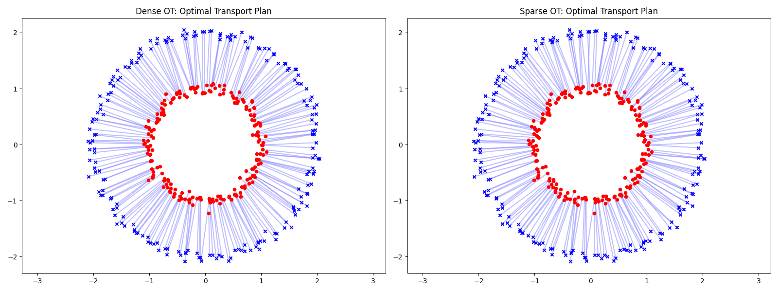
Dense OT cost: 0.992179
Sparse OT cost: 0.992290