Plot partial FGW for subgraph matching

This example illustrates the computation of partial (Fused) Gromov-Wasserstein divergences for subgraph matching tasks, using the exact formulation $p(F)GW$ and the entropically regularized one $p(F)GW_e$ [18, 29].

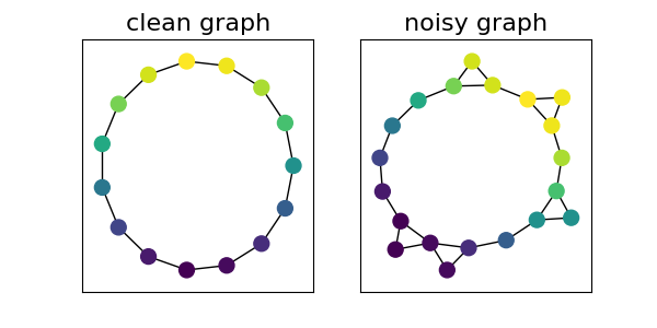
We first create a clean circular graph of 15 nodes with node features correlated with node positions on the unit circle, and a noisy version where 5 nodes out of the circle are added. Then knowing the proportion of clean samples in the target graph $m=3/4$, we show how to identify them using :

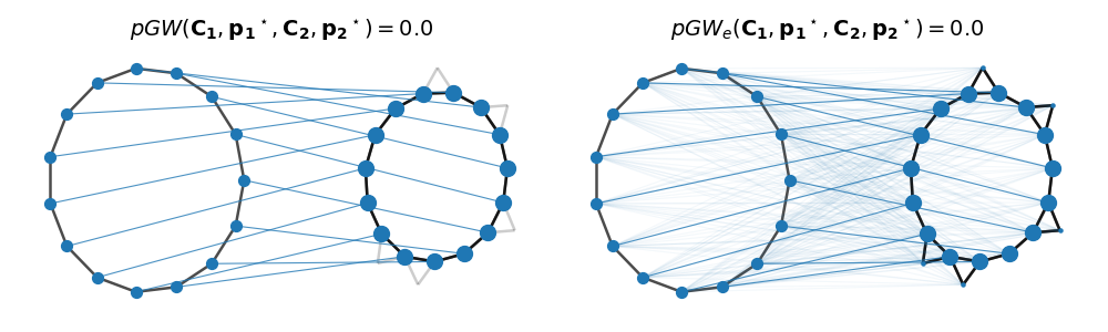
• The partial GW matching and its entropic counterpart, omitting node features.

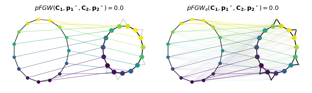
• The partial Fused GW matching and its entropic counterpart.

[18] Vayer Titouan, Chapel Laetitia, Flamary Rémi, Tavenard Romain and Courty Nicolas “Optimal Transport for structured data with application on graphs” International Conference on Machine Learning (ICML). 2019.

[29] Chapel, L., Alaya, M., Gasso, G. (2020). “Partial Optimal Transport with Applications on Positive-Unlabeled Learning”. NeurIPS.

# Author: Cédric Vincent-Cuaz <cedvincentcuaz@gmail.com>
#
# License: MIT License

# sphinx_gallery_thumbnail_number = 3

import numpy as np
import pylab as pl
import networkx as nx
import math
from scipy.sparse.csgraph import shortest_path
import matplotlib.colors as mcol
from matplotlib import cm
from ot.gromov import (
    partial_gromov_wasserstein,
    entropic_partial_gromov_wasserstein,
    partial_fused_gromov_wasserstein,
    entropic_partial_fused_gromov_wasserstein,
)
from ot import unif, dist

Utils for generation and visualization

def build_noisy_circular_graph(n_clean=15, n_noise=5, random_seed=0):
    """Create a noisy circular graph"""
    # create clean circle
    np.random.seed(random_seed)
    g = nx.Graph()
    g.add_nodes_from(np.arange(n_clean + n_noise))
    for i in range(n_clean):
        g.add_node(i, weight=math.sin(2 * i * math.pi / n_clean))
        if i == (n_clean - 1):
            g.add_edge(i, 0)
        else:
            g.add_edge(i, i + 1)
    # add nodes out of the circle as structure noise
    if n_noise > 0:
        noisy_nodes = np.random.choice(np.arange(n_clean), n_noise)
        for i, j in enumerate(noisy_nodes):
            g.add_node(i + n_clean, weight=math.sin(2 * j * math.pi / n_clean))
            g.add_edge(i + n_clean, j)
            g.add_edge(i + n_clean, (j + 1) % n_clean)
    return g


def graph_colors(nx_graph, vmin=0, vmax=7):
    cnorm = mcol.Normalize(vmin=vmin, vmax=vmax)
    cpick = cm.ScalarMappable(norm=cnorm, cmap="viridis")
    cpick.set_array([])
    val_map = {}
    for k, v in nx.get_node_attributes(nx_graph, "weight").items():
        val_map[k] = cpick.to_rgba(v)
    colors = []
    for node in nx_graph.nodes():
        colors.append(val_map[node])
    return colors


def draw_graph(
    G,
    C,
    nodes_color_part,
    Gweights=None,
    pos=None,
    edge_color="black",
    node_size=None,
    shiftx=0,
):
    if pos is None:
        pos = nx.kamada_kawai_layout(G)

    if shiftx != 0:
        for k, v in pos.items():
            v[0] = v[0] + shiftx

    alpha_edge = 0.7
    width_edge = 1.8
    if Gweights is None:
        nx.draw_networkx_edges(
            G, pos, width=width_edge, alpha=alpha_edge, edge_color=edge_color
        )
    else:
        # We make more visible connections between activated nodes
        n = len(Gweights)
        edgelist_activated = []
        edgelist_deactivated = []
        for i in range(n):
            for j in range(n):
                if Gweights[i] * Gweights[j] * C[i, j] > 0:
                    edgelist_activated.append((i, j))
                elif C[i, j] > 0:
                    edgelist_deactivated.append((i, j))

        nx.draw_networkx_edges(
            G,
            pos,
            edgelist=edgelist_activated,
            width=width_edge,
            alpha=alpha_edge,
            edge_color=edge_color,
        )
        nx.draw_networkx_edges(
            G,
            pos,
            edgelist=edgelist_deactivated,
            width=width_edge,
            alpha=0.1,
            edge_color=edge_color,
        )

    if Gweights is None:
        for node, node_color in enumerate(nodes_color_part):
            nx.draw_networkx_nodes(
                G,
                pos,
                nodelist=[node],
                node_size=node_size,
                alpha=1,
                node_color=node_color,
            )
    else:
        scaled_Gweights = Gweights / (0.5 * Gweights.max())
        nodes_size = node_size * scaled_Gweights
        for node, node_color in enumerate(nodes_color_part):
            if nodes_size[node] == 0:
                local_node_size = 0
            else:
                local_node_size = max(0.1 * node_size, nodes_size[node])
            nx.draw_networkx_nodes(
                G,
                pos,
                nodelist=[node],
                node_size=local_node_size,
                alpha=1,
                node_color=node_color,
            )
    return pos


def draw_transp_colored(
    G1,
    C1,
    G2,
    C2,
    p1,
    p2,
    T,
    pos1=None,
    pos2=None,
    shiftx=4,
    switchx=False,
    node_size=70,
    color_features=False,
):
    if color_features:
        nodes_color_part1 = graph_colors(G1, vmin=-1, vmax=1)
        nodes_color_part2 = graph_colors(G2, vmin=-1, vmax=1)
    else:
        nodes_color_part1 = C1.shape[0] * ["C0"]
        nodes_color_part2 = C2.shape[0] * ["C0"]

    pos1 = draw_graph(
        G1,
        C1,
        nodes_color_part1,
        Gweights=p1,
        pos=pos1,
        node_size=node_size,
        shiftx=0,
    )
    pos2 = draw_graph(
        G2,
        C2,
        nodes_color_part2,
        Gweights=p2,
        pos=pos2,
        node_size=node_size,
        shiftx=shiftx,
    )
    T_max = T.max()
    for k1, v1 in pos1.items():
        for k2, v2 in pos2.items():
            if T[k1, k2] > 0:
                pl.plot(
                    [pos1[k1][0], pos2[k2][0]],
                    [pos1[k1][1], pos2[k2][1]],
                    "-",
                    lw=0.8,
                    alpha=max(0.05, 0.8 * T[k1, k2] / T_max),
                    color=nodes_color_part1[k1],
                )
    return pos1, pos2

Generate and visualize data

We build a clean circular graph that will be matched to a noisy circular graph.

clean_graph = build_noisy_circular_graph(n_clean=15, n_noise=0)

noisy_graph = build_noisy_circular_graph(n_clean=15, n_noise=5)

graphs = [clean_graph, noisy_graph]
list_pos = []
pl.figure(figsize=(6, 3))
for i in range(2):
    pl.subplot(1, 2, i + 1)
    g = graphs[i]
    if i == 0:
        pl.title("clean graph", fontsize=16)
    else:
        pl.title("noisy graph", fontsize=16)
    pos = nx.kamada_kawai_layout(g)
    list_pos.append(pos)
    nx.draw_networkx(
        g,
        pos=pos,
        node_color=graph_colors(g, vmin=-1, vmax=1),
        with_labels=False,
        node_size=100,
    )
pl.show()

Partial (Entropic) Gromov-Wasserstein computation and visualization

Adjacency matrices are compared using both exact and entropic partial GW discarding for now node features. Then for illustration, the node sizes are proportional to their optimized masses and the intensity of the link between two nodes across graphs is set proportionally to the corresponding transported mass.

Cs = [nx.adjacency_matrix(G).toarray().astype(np.float64) for G in graphs]
ps = [unif(C.shape[0]) for C in Cs]

# provide an informative initialization for better visualization
m = 3.0 / 4.0
partial_id = np.zeros((15, 20))
partial_id[:15, :15] = np.eye(15) / 15.0
G0 = (np.outer(ps[0], ps[1]) + partial_id) * m / 2

# compute exact partial GW
T, log = partial_gromov_wasserstein(
    Cs[0], Cs[1], ps[0], ps[1], m=m, G0=G0, symmetric=True, log=True
)

# compute entropic partial GW leading to dense transport plans
Tent, logent = entropic_partial_gromov_wasserstein(
    Cs[0], Cs[1], ps[0], ps[1], reg=0.01, m=m, G0=G0, symmetric=True, log=True
)

# Plot matchings
list_T = [T, Tent]
list_dist = [
    np.round(log["partial_gw_dist"], 3),
    np.round(logent["partial_gw_dist"], 3),
]
list_dist_str = ["pGW", "pGW_e"]

pl.figure(2, figsize=(10, 3))
pl.clf()
for i in range(2):
    pl.subplot(1, 2, i + 1)
    pl.axis("off")
    pl.title(
        r"$%s(\mathbf{C_1},\mathbf{p_1}^\star,\mathbf{C_2},\mathbf{p_2}^\star) =%s$"
        % (list_dist_str[i], list_dist[i]),
        fontsize=14,
    )

    p2 = list_T[i].sum(0)

    pos1, pos2 = draw_transp_colored(
        clean_graph,
        Cs[0],
        noisy_graph,
        Cs[1],
        p1=None,
        p2=p2,
        T=list_T[i],
        shiftx=3,
        node_size=50,
    )

pl.tight_layout()
pl.show()

Partial (Entropic) Fused Gromov-Wasserstein computation and visualization

We add now node features compared using pairwise euclidean distance to illustrate partial FGW computation with trade-off parameter alpha=0.5

Ys = [
    np.array([v for (k, v) in nx.get_node_attributes(G, "weight").items()]).reshape(
        -1, 1
    )
    for G in graphs
]
M = dist(Ys[0], Ys[1])
# provide an informative initialization for better visualization
m = 3.0 / 4.0
partial_id = np.zeros((15, 20))
partial_id[:15, :15] = np.eye(15) / 15.0
G0 = (np.outer(ps[0], ps[1]) + partial_id) * m / 2

# compute exact partial GW
T, log = partial_fused_gromov_wasserstein(
    M,
    Cs[0],
    Cs[1],
    ps[0],
    ps[1],
    alpha=0.5,
    m=m,
    G0=G0,
    symmetric=True,
    log=True,
)

# compute entropic partial GW leading to dense transport plans
Tent, logent = entropic_partial_fused_gromov_wasserstein(
    M,
    Cs[0],
    Cs[1],
    ps[0],
    ps[1],
    reg=0.01,
    alpha=0.5,
    m=m,
    G0=G0,
    symmetric=True,
    log=True,
)

# Plot matchings
list_T = [T, Tent]
list_dist = [
    np.round(log["partial_fgw_dist"], 3),
    np.round(logent["partial_fgw_dist"], 3),
]
list_dist_str = ["pFGW", "pFGW_e"]

pl.figure(3, figsize=(10, 3))
pl.clf()
for i in range(2):
    pl.subplot(1, 2, i + 1)
    pl.axis("off")
    pl.title(
        r"$%s(\mathbf{C_1},\mathbf{p_1}^\star,\mathbf{C_2}, \mathbf{p_2}^\star) =%s$"
        % (list_dist_str[i], list_dist[i]),
        fontsize=14,
    )

    p2 = list_T[i].sum(0)
    pos1, pos2 = draw_transp_colored(
        clean_graph,
        Cs[0],
        noisy_graph,
        Cs[1],
        p1=None,
        p2=p2,
        T=list_T[i],
        shiftx=3,
        node_size=50,
        color_features=True,
    )

pl.tight_layout()
pl.show()

/home/circleci/.local/lib/python3.10/site-packages/networkx/drawing/nx_pylab.py:457: UserWarning: *c* argument looks like a single numeric RGB or RGBA sequence, which should be avoided as value-mapping will have precedence in case its length matches with *x* & *y*.  Please use the *color* keyword-argument or provide a 2D array with a single row if you intend to specify the same RGB or RGBA value for all points.
  node_collection = ax.scatter(