ot.sgot

Spectral-Grassmann optimal transport for linear operators.

This module implements the Spectral-Grassmann Wasserstein framework for comparing dynamical systems via their learned operator representations.

It provides tools to extract spectral “atoms” (eigenvalues and associated eigenspaces) from linear operators and to compute an optimal transport metric that combines a spectral term on eigenvalues with a Grassmannian term on eigenspaces.

Functions

ot.sgot.eigenvalue_cost_matrix(Ds, Dt, q=1, eigen_scaling=None, nx=None)

Compute pairwise eigenvalue distances for source and target domains.

Parameters:

• Ds (array-like, shape (n_s,)) – Source eigenvalues.

• Dt (array-like, shape (n_t,)) – Target eigenvalues.

• q (int or float, optional) – Exponent applied to the eigenvalue distance, default 1.

• eigen_scaling (None or array-like of length 2, optional) – Scaling (real_scale, imag_scale) applied to eigenvalues before computing distances. If None, defaults to (1.0, 1.0). Accepts tuple/list or array/tensor with two entries.

• nx (module, optional) – Backend (NumPy-compatible). If None, inferred from inputs.

Returns:

C – Eigenvalue cost matrix.

Return type:

np.ndarray, shape (n_s, n_t)

ot.sgot.sgot_cost_matrix(Ds, Rs, Ls, Dt, Rt, Lt, eta=0.5, p=2, q=1, grassmann_metric='chordal', eigen_scaling=None, nx=None, eps=1e-12)

Compute the SGOT cost matrix between two spectral decompositions.

This returns the discrete ground cost matrix used in the SGOT optimal transport objective. Each spectral atom is \(z_i=(\lambda_i, V_i)\) where \(\lambda_i \in \mathbb{C}\) is an eigenvalue and \(V_i\) is the associated (bi-orthogonal) eigenspace point.

\[C_2(i,j) \;=\; \eta\,C_\lambda(i,j) \;+\; (1-\eta)\,C_G(i,j),\]

with spectral term

\[C_\lambda(i,j) \;=\; \big|\lambda_i - \lambda'_j\big|^{q},\]

and Grassmann term computed from a similarity score \(\delta_{ij}\in[0,1]\) built from left/right eigenvectors

\[\delta_{ij} \;=\; \left|\langle r_i, r'_j\rangle\,\langle \ell_i, \ell'_j\rangle\right|.\]

Depending on grassmann_metric, the Grassmann contribution is:

• "chordal": \(C_G(i,j) = 1 - \delta_{ij}^2\)

• "geodesic": \(C_G(i,j) = \arccos(\delta_{ij})^2\)

• "procrustes": \(C_G(i,j) = 2(1-\delta_{ij})\)

• "martin": \(C_G(i,j) = -\log\!\left(\max(\delta_{ij}^2,\varepsilon)\right)\)

Finally, we return a matrix suited for a \(p\)-Wasserstein objective by treating \(C_2 \approx d^2\) and outputting

\[C(i,j) \;=\; \big(\operatorname{Re}(C_2(i,j))\big)^{p/2}.\]

Parameters:

• Ds (array-like, shape (n_s,)) – Eigenvalues of operator T1.

• Rs (array-like, shape (L, n_s)) – Right eigenvectors of operator T1.

• Ls (array-like, shape (L, n_s)) – Left eigenvectors of operator T1.

• Dt (array-like, shape (n_t,)) – Eigenvalues of operator T2.

• Rt (array-like, shape (L, n_t)) – Right eigenvectors of operator T2.

• Lt (array-like, shape (L, n_t)) – Left eigenvectors of operator T2.

• eta (float, optional) – Weighting between spectral and Grassmann terms, default 0.5.

• p (int, optional) – Exponent defining the OT ground cost. The returned cost is \(d^p\) with \(d^2 \approx C_2\). Default is 2.

• q (int, optional) – Exponent applied to the eigenvalue distance in the spectral term. Default is 1.

• grassmann_metric (str, optional) – Metric type: “geodesic”, “chordal”, “procrustes”, or “martin”.

• eigen_scaling (None or array-like of length 2, optional) – Scaling (real_scale, imag_scale) applied to eigenvalues before computing \(C_\lambda\). If provided, eigenvalues are transformed as \(\lambda \mapsto \alpha\operatorname{Re}(\lambda) + i\,\beta\operatorname{Im}(\lambda)\). If None, defaults to (1.0, 1.0). Accepts tuple/list or array/tensor with two entries.

• nx (module, optional) – Backend (NumPy-compatible). If None, inferred from inputs.

• eps (float, optional) – Minimum value used for numerical stability in Grassmann distances and Martin metric. Default is 1e-12.

Returns:

C – SGOT cost matrix \(C = d^p\).

Return type:

array-like, shape (n_s, n_t)

References

[83]

Germain, T., Flamary, R., Kostic, V. R., & Lounici, K. (2025). A Spectral-Grassmann Wasserstein Metric for Operator Representations of Dynamical Systems.

ot.sgot.sgot_metric(Ds, Rs, Ls, Dt, Rt, Lt, eta=0.5, p=2, q=1, r=2, grassmann_metric='chordal', eigen_scaling=None, Ws=None, Wt=None, nx=None, eps=1e-12)

Compute the SGOT metric between two spectral decompositions.

This function computes a discrete optimal transport problem between two measures over spectral atoms \(z_i=(\lambda_i, V_i)\) and \(z'_j=(\lambda'_j, V'_j)\). Using the ground cost matrix \(C = d^p\) returned by sgot_cost_matrix(), we solve:

\[P^\star \in \arg\min_{P\in\Pi(W_s, W_t)} \langle C, P\rangle,\]

where \(C(i,j) = d(i,j)^p\) and \(d(i,j)\) is the SGOT ground distance combining spectral and Grassmann terms with exponent \(q\):

\[d(i,j)^2 \;=\; \eta\,\big|\lambda_i - \lambda'_j\big|^{q} \;+\; (1-\eta)\,d_G(i,j)^{q},\]

and \(d_G(i,j)\) is the Grassmann distance associated with the chosen grassmann_metric.

From the optimal plan \(P^\star\), we first form the \(p\)-Wasserstein objective:

\[\mathrm{obj} \;=\; \left(\sum_{i,j} C(i,j)\,P^\star_{ij}\right)^{1/p},\]

and then apply an outer root \(r\):

\[\mathrm{SGOT} \;=\; \mathrm{obj}^{1/r}.\]

In summary:

• \(q\) controls how strongly spectral and Grassmann distances are curved (via \(|\lambda_i - \lambda'_j|^{q}\) and \(d_G(i,j)^{q}\)),

• \(p\) is the exponent used in the OT ground cost and the inner Wasserstein root,

• \(r\) is an additional outer root applied to the Wasserstein objective.

Parameters:

• Ds (array-like, shape (n_s,)) – Eigenvalues of operator T1.

• Rs (array-like, shape (L, n_s)) – Right eigenvectors of operator T1.

• Ls (array-like, shape (L, n_s)) – Left eigenvectors of operator T1.

• Dt (array-like, shape (n_t,)) – Eigenvalues of operator T2.

• Rt (array-like, shape (L, n_t)) – Right eigenvectors of operator T2.

• Lt (array-like, shape (L, n_t)) – Left eigenvectors of operator T2.

• eta (float, optional) – Weighting between spectral and Grassmann terms, default 0.5.

• p (int, optional) – Exponent defining the OT ground cost, default 2.

• q (int, optional) – Exponent applied to the eigenvalue and Grassmann distances, default 1.

• r (int or float, optional) – Outer root applied to the Wasserstein objective, default 2.

• grassmann_metric (str, optional) – Metric type: “geodesic”, “chordal”, “procrustes”, or “martin”.

• eigen_scaling (None or array-like of length 2, optional) – Scaling (real_scale, imag_scale) applied to eigenvalues before computing the spectral cost. If None, defaults to (1.0, 1.0).

• Ws (array-like, shape (n_s,), optional) – Source weights. If None, uniform weights are used.

• Wt (array-like, shape (n_t,), optional) – Target weights. If None, uniform weights are used.

• nx (module, optional) – Backend (NumPy-compatible). If None, inferred from inputs.

• eps (float, optional) – Numerical stability constant, default 1e-12.

Returns:

dist – SGOT distance between the two spectral decompositions.

Return type:

float

References

[83]

Germain, T., Flamary, R., Kostic, V. R., & Lounici, K. (2025). A Spectral-Grassmann Wasserstein Metric for Operator Representations of Dynamical Systems.

Examples using ot.sgot.sgot_metric

Spectral-Grassmann OT on dynamical systems operators

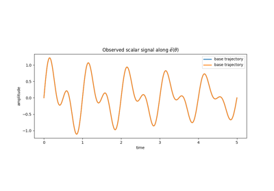
Spectral-Grassmann OT on dynamical systems operators

ot.sgot.eigenvalue_cost_matrix(Ds, Dt, q=1, eigen_scaling=None, nx=None)

Compute pairwise eigenvalue distances for source and target domains.

Parameters:

• Ds (array-like, shape (n_s,)) – Source eigenvalues.

• Dt (array-like, shape (n_t,)) – Target eigenvalues.

• q (int or float, optional) – Exponent applied to the eigenvalue distance, default 1.

• eigen_scaling (None or array-like of length 2, optional) – Scaling (real_scale, imag_scale) applied to eigenvalues before computing distances. If None, defaults to (1.0, 1.0). Accepts tuple/list or array/tensor with two entries.

• nx (module, optional) – Backend (NumPy-compatible). If None, inferred from inputs.

Returns:

C – Eigenvalue cost matrix.

Return type:

np.ndarray, shape (n_s, n_t)

ot.sgot.sgot_cost_matrix(Ds, Rs, Ls, Dt, Rt, Lt, eta=0.5, p=2, q=1, grassmann_metric='chordal', eigen_scaling=None, nx=None, eps=1e-12)

Compute the SGOT cost matrix between two spectral decompositions.

This returns the discrete ground cost matrix used in the SGOT optimal transport objective. Each spectral atom is \(z_i=(\lambda_i, V_i)\) where \(\lambda_i \in \mathbb{C}\) is an eigenvalue and \(V_i\) is the associated (bi-orthogonal) eigenspace point.

\[C_2(i,j) \;=\; \eta\,C_\lambda(i,j) \;+\; (1-\eta)\,C_G(i,j),\]

with spectral term

\[C_\lambda(i,j) \;=\; \big|\lambda_i - \lambda'_j\big|^{q},\]

and Grassmann term computed from a similarity score \(\delta_{ij}\in[0,1]\) built from left/right eigenvectors

\[\delta_{ij} \;=\; \left|\langle r_i, r'_j\rangle\,\langle \ell_i, \ell'_j\rangle\right|.\]

Depending on grassmann_metric, the Grassmann contribution is:

• "chordal": \(C_G(i,j) = 1 - \delta_{ij}^2\)

• "geodesic": \(C_G(i,j) = \arccos(\delta_{ij})^2\)

• "procrustes": \(C_G(i,j) = 2(1-\delta_{ij})\)

• "martin": \(C_G(i,j) = -\log\!\left(\max(\delta_{ij}^2,\varepsilon)\right)\)

Finally, we return a matrix suited for a \(p\)-Wasserstein objective by treating \(C_2 \approx d^2\) and outputting

\[C(i,j) \;=\; \big(\operatorname{Re}(C_2(i,j))\big)^{p/2}.\]

Parameters:

• Ds (array-like, shape (n_s,)) – Eigenvalues of operator T1.

• Rs (array-like, shape (L, n_s)) – Right eigenvectors of operator T1.

• Ls (array-like, shape (L, n_s)) – Left eigenvectors of operator T1.

• Dt (array-like, shape (n_t,)) – Eigenvalues of operator T2.

• Rt (array-like, shape (L, n_t)) – Right eigenvectors of operator T2.

• Lt (array-like, shape (L, n_t)) – Left eigenvectors of operator T2.

• eta (float, optional) – Weighting between spectral and Grassmann terms, default 0.5.

• p (int, optional) – Exponent defining the OT ground cost. The returned cost is \(d^p\) with \(d^2 \approx C_2\). Default is 2.

• q (int, optional) – Exponent applied to the eigenvalue distance in the spectral term. Default is 1.

• grassmann_metric (str, optional) – Metric type: “geodesic”, “chordal”, “procrustes”, or “martin”.

• eigen_scaling (None or array-like of length 2, optional) – Scaling (real_scale, imag_scale) applied to eigenvalues before computing \(C_\lambda\). If provided, eigenvalues are transformed as \(\lambda \mapsto \alpha\operatorname{Re}(\lambda) + i\,\beta\operatorname{Im}(\lambda)\). If None, defaults to (1.0, 1.0). Accepts tuple/list or array/tensor with two entries.

• nx (module, optional) – Backend (NumPy-compatible). If None, inferred from inputs.

• eps (float, optional) – Minimum value used for numerical stability in Grassmann distances and Martin metric. Default is 1e-12.

Returns:

C – SGOT cost matrix \(C = d^p\).

Return type:

array-like, shape (n_s, n_t)

References

[83]

Germain, T., Flamary, R., Kostic, V. R., & Lounici, K. (2025). A Spectral-Grassmann Wasserstein Metric for Operator Representations of Dynamical Systems.

ot.sgot.sgot_metric(Ds, Rs, Ls, Dt, Rt, Lt, eta=0.5, p=2, q=1, r=2, grassmann_metric='chordal', eigen_scaling=None, Ws=None, Wt=None, nx=None, eps=1e-12)

Compute the SGOT metric between two spectral decompositions.

This function computes a discrete optimal transport problem between two measures over spectral atoms \(z_i=(\lambda_i, V_i)\) and \(z'_j=(\lambda'_j, V'_j)\). Using the ground cost matrix \(C = d^p\) returned by sgot_cost_matrix(), we solve:

\[P^\star \in \arg\min_{P\in\Pi(W_s, W_t)} \langle C, P\rangle,\]

where \(C(i,j) = d(i,j)^p\) and \(d(i,j)\) is the SGOT ground distance combining spectral and Grassmann terms with exponent \(q\):

\[d(i,j)^2 \;=\; \eta\,\big|\lambda_i - \lambda'_j\big|^{q} \;+\; (1-\eta)\,d_G(i,j)^{q},\]

and \(d_G(i,j)\) is the Grassmann distance associated with the chosen grassmann_metric.

From the optimal plan \(P^\star\), we first form the \(p\)-Wasserstein objective:

\[\mathrm{obj} \;=\; \left(\sum_{i,j} C(i,j)\,P^\star_{ij}\right)^{1/p},\]

and then apply an outer root \(r\):

\[\mathrm{SGOT} \;=\; \mathrm{obj}^{1/r}.\]

In summary:

• \(q\) controls how strongly spectral and Grassmann distances are curved (via \(|\lambda_i - \lambda'_j|^{q}\) and \(d_G(i,j)^{q}\)),

• \(p\) is the exponent used in the OT ground cost and the inner Wasserstein root,

• \(r\) is an additional outer root applied to the Wasserstein objective.

Parameters:

• Ds (array-like, shape (n_s,)) – Eigenvalues of operator T1.

• Rs (array-like, shape (L, n_s)) – Right eigenvectors of operator T1.

• Ls (array-like, shape (L, n_s)) – Left eigenvectors of operator T1.

• Dt (array-like, shape (n_t,)) – Eigenvalues of operator T2.

• Rt (array-like, shape (L, n_t)) – Right eigenvectors of operator T2.

• Lt (array-like, shape (L, n_t)) – Left eigenvectors of operator T2.

• eta (float, optional) – Weighting between spectral and Grassmann terms, default 0.5.

• p (int, optional) – Exponent defining the OT ground cost, default 2.

• q (int, optional) – Exponent applied to the eigenvalue and Grassmann distances, default 1.

• r (int or float, optional) – Outer root applied to the Wasserstein objective, default 2.

• grassmann_metric (str, optional) – Metric type: “geodesic”, “chordal”, “procrustes”, or “martin”.

• eigen_scaling (None or array-like of length 2, optional) – Scaling (real_scale, imag_scale) applied to eigenvalues before computing the spectral cost. If None, defaults to (1.0, 1.0).

• Ws (array-like, shape (n_s,), optional) – Source weights. If None, uniform weights are used.

• Wt (array-like, shape (n_t,), optional) – Target weights. If None, uniform weights are used.

• nx (module, optional) – Backend (NumPy-compatible). If None, inferred from inputs.

• eps (float, optional) – Numerical stability constant, default 1e-12.

Returns:

dist – SGOT distance between the two spectral decompositions.

Return type:

float

References

[83]

Germain, T., Flamary, R., Kostic, V. R., & Lounici, K. (2025). A Spectral-Grassmann Wasserstein Metric for Operator Representations of Dynamical Systems.