ot.coot
CO-Optimal Transport solver
Functions
- ot.coot.co_optimal_transport(X, Y, wx_samp=None, wx_feat=None, wy_samp=None, wy_feat=None, epsilon=0, alpha=0, M_samp=None, M_feat=None, warmstart=None, nits_bcd=100, tol_bcd=1e-07, eval_bcd=1, nits_ot=500, tol_sinkhorn=1e-07, method_sinkhorn='sinkhorn', early_stopping_tol=1e-06, log=False, verbose=False)[source]
Compute the CO-Optimal Transport between two matrices.
Return the sample and feature transport plans between \((\mathbf{X}, \mathbf{w}_{xs}, \mathbf{w}_{xf})\) and \((\mathbf{Y}, \mathbf{w}_{ys}, \mathbf{w}_{yf})\).
The function solves the following CO-Optimal Transport (COOT) problem:
\[\begin{split}\mathbf{COOT}_{\alpha, \varepsilon} = \mathop{\arg \min}_{\mathbf{P}, \mathbf{Q}} &\quad \sum_{i,j,k,l} (\mathbf{X}_{i,k} - \mathbf{Y}_{j,l})^2 \mathbf{P}_{i,j} \mathbf{Q}_{k,l} + \alpha_s \sum_{i,j} \mathbf{P}_{i,j} \mathbf{M^{(s)}}_{i, j} \\ &+ \alpha_f \sum_{k, l} \mathbf{Q}_{k,l} \mathbf{M^{(f)}}_{k, l} + \varepsilon_s \mathbf{KL}(\mathbf{P} | \mathbf{w}_{xs} \mathbf{w}_{ys}^T) + \varepsilon_f \mathbf{KL}(\mathbf{Q} | \mathbf{w}_{xf} \mathbf{w}_{yf}^T)\end{split}\]Where :
\(\mathbf{X}\): Data matrix in the source space
\(\mathbf{Y}\): Data matrix in the target space
\(\mathbf{M^{(s)}}\): Additional sample matrix
\(\mathbf{M^{(f)}}\): Additional feature matrix
\(\mathbf{w}_{xs}\): Distribution of the samples in the source space
\(\mathbf{w}_{xf}\): Distribution of the features in the source space
\(\mathbf{w}_{ys}\): Distribution of the samples in the target space
\(\mathbf{w}_{yf}\): Distribution of the features in the target space
Note
This function allows epsilon to be zero. In that case, the
ot.lp.emdsolver of POT will be used.- Parameters:
X ((n_sample_x, n_feature_x) array-like, float) – First input matrix.
Y ((n_sample_y, n_feature_y) array-like, float) – Second input matrix.
wx_samp ((n_sample_x, ) array-like, float, optional (default = None)) – Histogram assigned on rows (samples) of matrix X. Uniform distribution by default.
wx_feat ((n_feature_x, ) array-like, float, optional (default = None)) – Histogram assigned on columns (features) of matrix X. Uniform distribution by default.
wy_samp ((n_sample_y, ) array-like, float, optional (default = None)) – Histogram assigned on rows (samples) of matrix Y. Uniform distribution by default.
wy_feat ((n_feature_y, ) array-like, float, optional (default = None)) – Histogram assigned on columns (features) of matrix Y. Uniform distribution by default.
epsilon (scalar or indexable object of length 2, float or int, optional (default = 0)) – Regularization parameters for entropic approximation of sample and feature couplings. Allow the case where epsilon contains 0. In that case, the EMD solver is used instead of Sinkhorn solver. If epsilon is scalar, then the same epsilon is applied to both regularization of sample and feature couplings.
alpha (scalar or indexable object of length 2, float or int, optional (default = 0)) – Coefficient parameter of linear terms with respect to the sample and feature couplings. If alpha is scalar, then the same alpha is applied to both linear terms.
M_samp ((n_sample_x, n_sample_y), float, optional (default = None)) – Sample matrix with respect to the linear term on sample coupling.
M_feat ((n_feature_x, n_feature_y), float, optional (default = None)) – Feature matrix with respect to the linear term on feature coupling.
warmstart (dictionary, optional (default = None)) –
- Contains 4 keys:
”duals_sample” and “duals_feature” whose values are tuples of 2 vectors of size (n_sample_x, n_sample_y) and (n_feature_x, n_feature_y). Initialization of sample and feature dual vectors if using Sinkhorn algorithm. Zero vectors by default.
”pi_sample” and “pi_feature” whose values are matrices of size (n_sample_x, n_sample_y) and (n_feature_x, n_feature_y). Initialization of sample and feature couplings. Uniform distributions by default.
nits_bcd (int, optional (default = 100)) – Number of Block Coordinate Descent (BCD) iterations to solve COOT.
tol_bcd (float, optional (default = 1e-7)) – Tolerance of BCD scheme. If the L1-norm between the current and previous sample couplings is under this threshold, then stop BCD scheme.
eval_bcd (int, optional (default = 1)) – Multiplier of iteration at which the COOT cost is evaluated. For example, if eval_bcd = 8, then the cost is calculated at iterations 8, 16, 24, etc…
nits_ot (int, optional (default = 100)) – Number of iterations to solve each of the two optimal transport problems in each BCD iteration.
tol_sinkhorn (float, optional (default = 1e-7)) – Tolerance of Sinkhorn algorithm to stop the Sinkhorn scheme for entropic optimal transport problem (if any) in each BCD iteration. Only triggered when Sinkhorn solver is used.
method_sinkhorn (string, optional (default = "sinkhorn")) – Method used in POT’s ot.sinkhorn solver. Only support “sinkhorn” and “sinkhorn_log”.
early_stopping_tol (float, optional (default = 1e-6)) – Tolerance for the early stopping. If the absolute difference between the last 2 recorded COOT distances is under this tolerance, then stop BCD scheme.
log (bool, optional (default = False)) – If True then the cost and 4 dual vectors, including 2 from sample and 2 from feature couplings, are recorded.
verbose (bool, optional (default = False)) – If True then print the COOT cost at every multiplier of eval_bcd-th iteration.
- Returns:
pi_samp ((n_sample_x, n_sample_y) array-like, float) – Sample coupling matrix.
pi_feat ((n_feature_x, n_feature_y) array-like, float) – Feature coupling matrix.
log (dictionary, optional) –
- Returned if log is True. The keys are:
- duals_sample(n_sample_x, n_sample_y) tuple, float
Pair of dual vectors when solving OT problem w.r.t the sample coupling.
- duals_feature(n_feature_x, n_feature_y) tuple, float
Pair of dual vectors when solving OT problem w.r.t the feature coupling.
- distanceslist, float
List of COOT distances along iterations.
References
Examples using ot.coot.co_optimal_transport
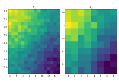
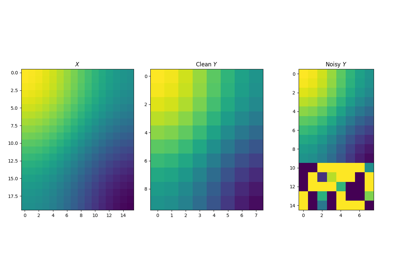
Row and column alignments with CO-Optimal Transport
- ot.coot.co_optimal_transport2(X, Y, wx_samp=None, wx_feat=None, wy_samp=None, wy_feat=None, epsilon=0, alpha=0, M_samp=None, M_feat=None, warmstart=None, log=False, verbose=False, early_stopping_tol=1e-06, nits_bcd=100, tol_bcd=1e-07, eval_bcd=1, nits_ot=500, tol_sinkhorn=1e-07, method_sinkhorn='sinkhorn')[source]
Compute the CO-Optimal Transport distance between two measures.
Returns the CO-Optimal Transport distance between \((\mathbf{X}, \mathbf{w}_{xs}, \mathbf{w}_{xf})\) and \((\mathbf{Y}, \mathbf{w}_{ys}, \mathbf{w}_{yf})\).
The function solves the following CO-Optimal Transport (COOT) problem:
\[\begin{split}\mathbf{COOT}_{\alpha, \varepsilon} = \mathop{\arg \min}_{\mathbf{P}, \mathbf{Q}} &\quad \sum_{i,j,k,l} (\mathbf{X}_{i,k} - \mathbf{Y}_{j,l})^2 \mathbf{P}_{i,j} \mathbf{Q}_{k,l} + \alpha_1 \sum_{i,j} \mathbf{P}_{i,j} \mathbf{M^{(s)}}_{i, j} \\ &+ \alpha_2 \sum_{k, l} \mathbf{Q}_{k,l} \mathbf{M^{(f)}}_{k, l} + \varepsilon_1 \mathbf{KL}(\mathbf{P} | \mathbf{w}_{xs} \mathbf{w}_{ys}^T) + \varepsilon_2 \mathbf{KL}(\mathbf{Q} | \mathbf{w}_{xf} \mathbf{w}_{yf}^T)\end{split}\]where :
\(\mathbf{X}\): Data matrix in the source space
\(\mathbf{Y}\): Data matrix in the target space
\(\mathbf{M^{(s)}}\): Additional sample matrix
\(\mathbf{M^{(f)}}\): Additional feature matrix
\(\mathbf{w}_{xs}\): Distribution of the samples in the source space
\(\mathbf{w}_{xf}\): Distribution of the features in the source space
\(\mathbf{w}_{ys}\): Distribution of the samples in the target space
\(\mathbf{w}_{yf}\): Distribution of the features in the target space
Note
This function allows epsilon to be zero. In that case, the
ot.lp.emdsolver of POT will be used.- Parameters:
X ((n_sample_x, n_feature_x) array-like, float) – First input matrix.
Y ((n_sample_y, n_feature_y) array-like, float) – Second input matrix.
wx_samp ((n_sample_x, ) array-like, float, optional (default = None)) – Histogram assigned on rows (samples) of matrix X. Uniform distribution by default.
wx_feat ((n_feature_x, ) array-like, float, optional (default = None)) – Histogram assigned on columns (features) of matrix X. Uniform distribution by default.
wy_samp ((n_sample_y, ) array-like, float, optional (default = None)) – Histogram assigned on rows (samples) of matrix Y. Uniform distribution by default.
wy_feat ((n_feature_y, ) array-like, float, optional (default = None)) – Histogram assigned on columns (features) of matrix Y. Uniform distribution by default.
epsilon (scalar or indexable object of length 2, float or int, optional (default = 0)) – Regularization parameters for entropic approximation of sample and feature couplings. Allow the case where epsilon contains 0. In that case, the EMD solver is used instead of Sinkhorn solver. If epsilon is scalar, then the same epsilon is applied to both regularization of sample and feature couplings.
alpha (scalar or indexable object of length 2, float or int, optional (default = 0)) – Coefficient parameter of linear terms with respect to the sample and feature couplings. If alpha is scalar, then the same alpha is applied to both linear terms.
M_samp ((n_sample_x, n_sample_y), float, optional (default = None)) – Sample matrix with respect to the linear term on sample coupling.
M_feat ((n_feature_x, n_feature_y), float, optional (default = None)) – Feature matrix with respect to the linear term on feature coupling.
warmstart (dictionary, optional (default = None)) –
- Contains 4 keys:
”duals_sample” and “duals_feature” whose values are tuples of 2 vectors of size (n_sample_x, n_sample_y) and (n_feature_x, n_feature_y). Initialization of sample and feature dual vectors if using Sinkhorn algorithm. Zero vectors by default.
”pi_sample” and “pi_feature” whose values are matrices of size (n_sample_x, n_sample_y) and (n_feature_x, n_feature_y). Initialization of sample and feature couplings. Uniform distributions by default.
nits_bcd (int, optional (default = 100)) – Number of Block Coordinate Descent (BCD) iterations to solve COOT.
tol_bcd (float, optional (default = 1e-7)) – Tolerance of BCD scheme. If the L1-norm between the current and previous sample couplings is under this threshold, then stop BCD scheme.
eval_bcd (int, optional (default = 1)) – Multiplier of iteration at which the COOT cost is evaluated. For example, if eval_bcd = 8, then the cost is calculated at iterations 8, 16, 24, etc…
nits_ot (int, optional (default = 100)) – Number of iterations to solve each of the two optimal transport problems in each BCD iteration.
tol_sinkhorn (float, optional (default = 1e-7)) – Tolerance of Sinkhorn algorithm to stop the Sinkhorn scheme for entropic optimal transport problem (if any) in each BCD iteration. Only triggered when Sinkhorn solver is used.
method_sinkhorn (string, optional (default = "sinkhorn")) – Method used in POT’s ot.sinkhorn solver. Only support “sinkhorn” and “sinkhorn_log”.
early_stopping_tol (float, optional (default = 1e-6)) – Tolerance for the early stopping. If the absolute difference between the last 2 recorded COOT distances is under this tolerance, then stop BCD scheme.
log (bool, optional (default = False)) – If True then the cost and 4 dual vectors, including 2 from sample and 2 from feature couplings, are recorded.
verbose (bool, optional (default = False)) – If True then print the COOT cost at every multiplier of eval_bcd-th iteration.
- Returns:
float – CO-Optimal Transport distance.
dict – Contains logged information from
co_optimal_transportsolver. Only returned if log parameter is True
References
Examples using ot.coot.co_optimal_transport2
Row and column alignments with CO-Optimal Transport
- ot.coot.co_optimal_transport(X, Y, wx_samp=None, wx_feat=None, wy_samp=None, wy_feat=None, epsilon=0, alpha=0, M_samp=None, M_feat=None, warmstart=None, nits_bcd=100, tol_bcd=1e-07, eval_bcd=1, nits_ot=500, tol_sinkhorn=1e-07, method_sinkhorn='sinkhorn', early_stopping_tol=1e-06, log=False, verbose=False)[source]
Compute the CO-Optimal Transport between two matrices.
Return the sample and feature transport plans between \((\mathbf{X}, \mathbf{w}_{xs}, \mathbf{w}_{xf})\) and \((\mathbf{Y}, \mathbf{w}_{ys}, \mathbf{w}_{yf})\).
The function solves the following CO-Optimal Transport (COOT) problem:
\[\begin{split}\mathbf{COOT}_{\alpha, \varepsilon} = \mathop{\arg \min}_{\mathbf{P}, \mathbf{Q}} &\quad \sum_{i,j,k,l} (\mathbf{X}_{i,k} - \mathbf{Y}_{j,l})^2 \mathbf{P}_{i,j} \mathbf{Q}_{k,l} + \alpha_s \sum_{i,j} \mathbf{P}_{i,j} \mathbf{M^{(s)}}_{i, j} \\ &+ \alpha_f \sum_{k, l} \mathbf{Q}_{k,l} \mathbf{M^{(f)}}_{k, l} + \varepsilon_s \mathbf{KL}(\mathbf{P} | \mathbf{w}_{xs} \mathbf{w}_{ys}^T) + \varepsilon_f \mathbf{KL}(\mathbf{Q} | \mathbf{w}_{xf} \mathbf{w}_{yf}^T)\end{split}\]Where :
\(\mathbf{X}\): Data matrix in the source space
\(\mathbf{Y}\): Data matrix in the target space
\(\mathbf{M^{(s)}}\): Additional sample matrix
\(\mathbf{M^{(f)}}\): Additional feature matrix
\(\mathbf{w}_{xs}\): Distribution of the samples in the source space
\(\mathbf{w}_{xf}\): Distribution of the features in the source space
\(\mathbf{w}_{ys}\): Distribution of the samples in the target space
\(\mathbf{w}_{yf}\): Distribution of the features in the target space
Note
This function allows epsilon to be zero. In that case, the
ot.lp.emdsolver of POT will be used.- Parameters:
X ((n_sample_x, n_feature_x) array-like, float) – First input matrix.
Y ((n_sample_y, n_feature_y) array-like, float) – Second input matrix.
wx_samp ((n_sample_x, ) array-like, float, optional (default = None)) – Histogram assigned on rows (samples) of matrix X. Uniform distribution by default.
wx_feat ((n_feature_x, ) array-like, float, optional (default = None)) – Histogram assigned on columns (features) of matrix X. Uniform distribution by default.
wy_samp ((n_sample_y, ) array-like, float, optional (default = None)) – Histogram assigned on rows (samples) of matrix Y. Uniform distribution by default.
wy_feat ((n_feature_y, ) array-like, float, optional (default = None)) – Histogram assigned on columns (features) of matrix Y. Uniform distribution by default.
epsilon (scalar or indexable object of length 2, float or int, optional (default = 0)) – Regularization parameters for entropic approximation of sample and feature couplings. Allow the case where epsilon contains 0. In that case, the EMD solver is used instead of Sinkhorn solver. If epsilon is scalar, then the same epsilon is applied to both regularization of sample and feature couplings.
alpha (scalar or indexable object of length 2, float or int, optional (default = 0)) – Coefficient parameter of linear terms with respect to the sample and feature couplings. If alpha is scalar, then the same alpha is applied to both linear terms.
M_samp ((n_sample_x, n_sample_y), float, optional (default = None)) – Sample matrix with respect to the linear term on sample coupling.
M_feat ((n_feature_x, n_feature_y), float, optional (default = None)) – Feature matrix with respect to the linear term on feature coupling.
warmstart (dictionary, optional (default = None)) –
- Contains 4 keys:
”duals_sample” and “duals_feature” whose values are tuples of 2 vectors of size (n_sample_x, n_sample_y) and (n_feature_x, n_feature_y). Initialization of sample and feature dual vectors if using Sinkhorn algorithm. Zero vectors by default.
”pi_sample” and “pi_feature” whose values are matrices of size (n_sample_x, n_sample_y) and (n_feature_x, n_feature_y). Initialization of sample and feature couplings. Uniform distributions by default.
nits_bcd (int, optional (default = 100)) – Number of Block Coordinate Descent (BCD) iterations to solve COOT.
tol_bcd (float, optional (default = 1e-7)) – Tolerance of BCD scheme. If the L1-norm between the current and previous sample couplings is under this threshold, then stop BCD scheme.
eval_bcd (int, optional (default = 1)) – Multiplier of iteration at which the COOT cost is evaluated. For example, if eval_bcd = 8, then the cost is calculated at iterations 8, 16, 24, etc…
nits_ot (int, optional (default = 100)) – Number of iterations to solve each of the two optimal transport problems in each BCD iteration.
tol_sinkhorn (float, optional (default = 1e-7)) – Tolerance of Sinkhorn algorithm to stop the Sinkhorn scheme for entropic optimal transport problem (if any) in each BCD iteration. Only triggered when Sinkhorn solver is used.
method_sinkhorn (string, optional (default = "sinkhorn")) – Method used in POT’s ot.sinkhorn solver. Only support “sinkhorn” and “sinkhorn_log”.
early_stopping_tol (float, optional (default = 1e-6)) – Tolerance for the early stopping. If the absolute difference between the last 2 recorded COOT distances is under this tolerance, then stop BCD scheme.
log (bool, optional (default = False)) – If True then the cost and 4 dual vectors, including 2 from sample and 2 from feature couplings, are recorded.
verbose (bool, optional (default = False)) – If True then print the COOT cost at every multiplier of eval_bcd-th iteration.
- Returns:
pi_samp ((n_sample_x, n_sample_y) array-like, float) – Sample coupling matrix.
pi_feat ((n_feature_x, n_feature_y) array-like, float) – Feature coupling matrix.
log (dictionary, optional) –
- Returned if log is True. The keys are:
- duals_sample(n_sample_x, n_sample_y) tuple, float
Pair of dual vectors when solving OT problem w.r.t the sample coupling.
- duals_feature(n_feature_x, n_feature_y) tuple, float
Pair of dual vectors when solving OT problem w.r.t the feature coupling.
- distanceslist, float
List of COOT distances along iterations.
References
- ot.coot.co_optimal_transport2(X, Y, wx_samp=None, wx_feat=None, wy_samp=None, wy_feat=None, epsilon=0, alpha=0, M_samp=None, M_feat=None, warmstart=None, log=False, verbose=False, early_stopping_tol=1e-06, nits_bcd=100, tol_bcd=1e-07, eval_bcd=1, nits_ot=500, tol_sinkhorn=1e-07, method_sinkhorn='sinkhorn')[source]
Compute the CO-Optimal Transport distance between two measures.
Returns the CO-Optimal Transport distance between \((\mathbf{X}, \mathbf{w}_{xs}, \mathbf{w}_{xf})\) and \((\mathbf{Y}, \mathbf{w}_{ys}, \mathbf{w}_{yf})\).
The function solves the following CO-Optimal Transport (COOT) problem:
\[\begin{split}\mathbf{COOT}_{\alpha, \varepsilon} = \mathop{\arg \min}_{\mathbf{P}, \mathbf{Q}} &\quad \sum_{i,j,k,l} (\mathbf{X}_{i,k} - \mathbf{Y}_{j,l})^2 \mathbf{P}_{i,j} \mathbf{Q}_{k,l} + \alpha_1 \sum_{i,j} \mathbf{P}_{i,j} \mathbf{M^{(s)}}_{i, j} \\ &+ \alpha_2 \sum_{k, l} \mathbf{Q}_{k,l} \mathbf{M^{(f)}}_{k, l} + \varepsilon_1 \mathbf{KL}(\mathbf{P} | \mathbf{w}_{xs} \mathbf{w}_{ys}^T) + \varepsilon_2 \mathbf{KL}(\mathbf{Q} | \mathbf{w}_{xf} \mathbf{w}_{yf}^T)\end{split}\]where :
\(\mathbf{X}\): Data matrix in the source space
\(\mathbf{Y}\): Data matrix in the target space
\(\mathbf{M^{(s)}}\): Additional sample matrix
\(\mathbf{M^{(f)}}\): Additional feature matrix
\(\mathbf{w}_{xs}\): Distribution of the samples in the source space
\(\mathbf{w}_{xf}\): Distribution of the features in the source space
\(\mathbf{w}_{ys}\): Distribution of the samples in the target space
\(\mathbf{w}_{yf}\): Distribution of the features in the target space
Note
This function allows epsilon to be zero. In that case, the
ot.lp.emdsolver of POT will be used.- Parameters:
X ((n_sample_x, n_feature_x) array-like, float) – First input matrix.
Y ((n_sample_y, n_feature_y) array-like, float) – Second input matrix.
wx_samp ((n_sample_x, ) array-like, float, optional (default = None)) – Histogram assigned on rows (samples) of matrix X. Uniform distribution by default.
wx_feat ((n_feature_x, ) array-like, float, optional (default = None)) – Histogram assigned on columns (features) of matrix X. Uniform distribution by default.
wy_samp ((n_sample_y, ) array-like, float, optional (default = None)) – Histogram assigned on rows (samples) of matrix Y. Uniform distribution by default.
wy_feat ((n_feature_y, ) array-like, float, optional (default = None)) – Histogram assigned on columns (features) of matrix Y. Uniform distribution by default.
epsilon (scalar or indexable object of length 2, float or int, optional (default = 0)) – Regularization parameters for entropic approximation of sample and feature couplings. Allow the case where epsilon contains 0. In that case, the EMD solver is used instead of Sinkhorn solver. If epsilon is scalar, then the same epsilon is applied to both regularization of sample and feature couplings.
alpha (scalar or indexable object of length 2, float or int, optional (default = 0)) – Coefficient parameter of linear terms with respect to the sample and feature couplings. If alpha is scalar, then the same alpha is applied to both linear terms.
M_samp ((n_sample_x, n_sample_y), float, optional (default = None)) – Sample matrix with respect to the linear term on sample coupling.
M_feat ((n_feature_x, n_feature_y), float, optional (default = None)) – Feature matrix with respect to the linear term on feature coupling.
warmstart (dictionary, optional (default = None)) –
- Contains 4 keys:
”duals_sample” and “duals_feature” whose values are tuples of 2 vectors of size (n_sample_x, n_sample_y) and (n_feature_x, n_feature_y). Initialization of sample and feature dual vectors if using Sinkhorn algorithm. Zero vectors by default.
”pi_sample” and “pi_feature” whose values are matrices of size (n_sample_x, n_sample_y) and (n_feature_x, n_feature_y). Initialization of sample and feature couplings. Uniform distributions by default.
nits_bcd (int, optional (default = 100)) – Number of Block Coordinate Descent (BCD) iterations to solve COOT.
tol_bcd (float, optional (default = 1e-7)) – Tolerance of BCD scheme. If the L1-norm between the current and previous sample couplings is under this threshold, then stop BCD scheme.
eval_bcd (int, optional (default = 1)) – Multiplier of iteration at which the COOT cost is evaluated. For example, if eval_bcd = 8, then the cost is calculated at iterations 8, 16, 24, etc…
nits_ot (int, optional (default = 100)) – Number of iterations to solve each of the two optimal transport problems in each BCD iteration.
tol_sinkhorn (float, optional (default = 1e-7)) – Tolerance of Sinkhorn algorithm to stop the Sinkhorn scheme for entropic optimal transport problem (if any) in each BCD iteration. Only triggered when Sinkhorn solver is used.
method_sinkhorn (string, optional (default = "sinkhorn")) – Method used in POT’s ot.sinkhorn solver. Only support “sinkhorn” and “sinkhorn_log”.
early_stopping_tol (float, optional (default = 1e-6)) – Tolerance for the early stopping. If the absolute difference between the last 2 recorded COOT distances is under this tolerance, then stop BCD scheme.
log (bool, optional (default = False)) – If True then the cost and 4 dual vectors, including 2 from sample and 2 from feature couplings, are recorded.
verbose (bool, optional (default = False)) – If True then print the COOT cost at every multiplier of eval_bcd-th iteration.
- Returns:
float – CO-Optimal Transport distance.
dict – Contains logged information from
co_optimal_transportsolver. Only returned if log parameter is True
References