Nyström approximation for OT

Shows how to use Nyström kernel approximation for approximating the Sinkhorn algorithm in linear time.

# Author: Titouan Vayer <titouan.vayer@inria.fr>
#
# License: MIT License

# sphinx_gallery_thumbnail_number = 2

import numpy as np
from ot.lowrank import kernel_nystroem, sinkhorn_low_rank_kernel
from ot.bregman import empirical_sinkhorn_nystroem
import math
import ot
import matplotlib.pyplot as plt
from matplotlib.colors import LogNorm

Generate data

offset = 1
n_samples_per_blob = 500  # We use 2D ''blobs'' data
random_state = 42
std = 0.2  # standard deviation
np.random.seed(random_state)

centers = np.array(
    [
        [-offset, -offset],  # Class 0 - blob 1
        [-offset, offset],  # Class 0 - blob 2
        [offset, -offset],  # Class 1 - blob 1
        [offset, offset],  # Class 1 - blob 2
    ]
)

X_list = []
y_list = []

for i, center in enumerate(centers):
    blob_points = np.random.randn(n_samples_per_blob, 2) * std + center
    label = 0 if i < 2 else 1
    X_list.append(blob_points)
    y_list.append(np.full(n_samples_per_blob, label))

X = np.vstack(X_list)
y = np.concatenate(y_list)
Xs = X[y == 0]  # source data
Xt = X[y == 1]  # target data

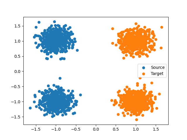
Plot data

plt.scatter(Xs[:, 0], Xs[:, 1], label="Source")
plt.scatter(Xt[:, 0], Xt[:, 1], label="Target")
plt.legend()

<matplotlib.legend.Legend object at 0x7f6b5e17d330>

Compute the Nyström approximation of the Gaussian kernel

reg = 5.0  # proportional to the std of the Gaussian kernel
anchors = 10  # number of anchor points for the Nyström approximation
ot.tic()
left_factor, right_factor = kernel_nystroem(
    Xs, Xt, anchors=anchors, sigma=math.sqrt(reg / 2.0), random_state=random_state
)
ot.toc()

Elapsed time : 0.0008536669993191026 s

0.0008536669993191026

Use this approximation in a Sinkhorn algorithm with low rank kernel. Each matrix/vector product in the Sinkhorn is accelerated since \(Kv = K_1 (K_2^\top v)\) can be computed in \(O(nr)\) time instead of \(O(n^2)\)

numItermax = 1000
stopThr = 1e-7
verbose = True
a, b = None, None
warn = True
warmstart = None
ot.tic()
u, v, dict_log = sinkhorn_low_rank_kernel(
    K1=left_factor,
    K2=right_factor,
    a=a,
    b=b,
    numItermax=numItermax,
    stopThr=stopThr,
    verbose=verbose,
    log=True,
    warn=warn,
    warmstart=warmstart,
)
ot.toc()

It.  |Err
-------------------
    0|7.482235e-05|
Elapsed time : 0.0010054979993583402 s

0.0010054979993583402

Compare with Sinkhorn

M = ot.dist(Xs, Xt)
ot.tic()
G, log_ = ot.sinkhorn(
    a=[],
    b=[],
    M=M,
    reg=reg,
    numItermax=numItermax,
    verbose=verbose,
    log=True,
    warn=warn,
    warmstart=warmstart,
)
ot.toc()

It.  |Err
-------------------
    0|7.517180e-05|
Elapsed time : 0.012269569999261876 s

0.012269569999261876

Use directly ot.bregman.empirical_sinkhorn_nystroem

ot.tic()
G_nys = empirical_sinkhorn_nystroem(
    Xs,
    Xt,
    anchors=anchors,
    reg=reg,
    numItermax=numItermax,
    verbose=True,
    random_state=random_state,
)[:]
ot.toc()

It.  |Err
-------------------
    0|7.482235e-05|
Elapsed time : 0.0033195709984283894 s

0.0033195709984283894

ot.tic()
G_sinkh = ot.bregman.empirical_sinkhorn(
    Xs, Xt, reg=reg, numIterMax=numItermax, verbose=True
)
ot.toc()

It.  |Err
-------------------
    0|7.517180e-05|
Elapsed time : 0.01705986200067855 s

0.01705986200067855

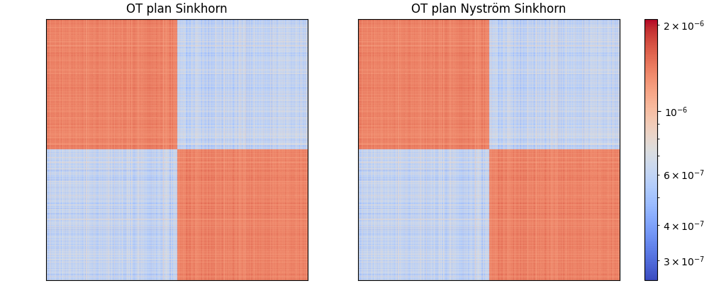
Compare OT plans

fig, ax = plt.subplots(1, 2, figsize=(10, 4), constrained_layout=True)
vmin = min(G_sinkh.min(), G_nys.min())
vmax = max(G_sinkh.max(), G_nys.max())
norm = LogNorm(vmin=vmin, vmax=vmax)
im0 = ax[0].imshow(G_sinkh, norm=norm, cmap="coolwarm")
im1 = ax[1].imshow(G_nys, norm=norm, cmap="coolwarm")
cbar = fig.colorbar(im1, ax=ax, orientation="vertical", fraction=0.046, pad=0.04)
ax[0].set_title("OT plan Sinkhorn")
ax[1].set_title("OT plan Nyström Sinkhorn")
for a in ax:
    a.set_xticks([])
    a.set_yticks([])
plt.show()